liuyujie0136's Website
A website for self learning, collecting and sharing.
R使用技巧
- R使用技巧
Statistics for Biologists - Nature Collection
Quick-R
修改RStudio的help文档样式
找到RStudio安装目录,一般为C:\Program Files\RStudio,打开resources文件夹,先备份R.css文件为R.css.bak,再用管理员权限将其替换为如下内容(可能需要在别处新建文件并写入内容再拷贝至该目录覆盖原文件):
/*
 * R.css
 *
 * Copyright (C) 2009-16 by RStudio, Inc.
 *
 * Unless you have received this program directly from RStudio pursuant
 * to the terms of a commercial license agreement with RStudio, then
 * this program is licensed to you under the terms of version 3 of the
 * GNU Affero General Public License. This program is distributed WITHOUT
 * ANY EXPRESS OR IMPLIED WARRANTY, INCLUDING THOSE OF NON-INFRINGEMENT,
 * MERCHANTABILITY OR FITNESS FOR A PARTICULAR PURPOSE. Please refer to the
 * AGPL (http://www.gnu.org/licenses/agpl-3.0.txt) for more details.
 *
 */

body, td {
   font-family: 'Source Sans Pro', 'Lucida Grande', Verdana, Arial, sans-serif !important;
   font-size: 15px !important;
}

body.macintosh, body.macintosh td {
   font-family: Consolas;
}

body.macintosh code,
body.macintosh pre {
   font-family: Consolas;
}

body code {
   font-family: Consolas;
}

::selection {
   background: rgb(181, 213, 255);
}

::-moz-selection{
   background: rgb(181, 213, 255);
}

a:visited {
   color: rgb(50%, 0%, 50%);
}

h1 {
   font-size: x-large;
}

h2 {
   font-size: x-large;
   font-weight: normal;
}

h3 {
   color: rgb(35%, 35%, 35%);
}

h4 {
   color: rgb(35%, 35%, 35%);
   font-style: italic;
}

h5 {
   color: rgb(35%, 35%, 35%);
}

h6 {
   color: rgb(35%, 35%, 35%);
   font-style: italic;
}

.rstudio-themes-flat.rstudio-themes-dark-grey h1,
.rstudio-themes-flat.rstudio-themes-dark-grey h2,
.rstudio-themes-flat.rstudio-themes-dark-grey h3,
.rstudio-themes-flat.rstudio-themes-dark-grey h4,
.rstudio-themes-flat.rstudio-themes-dark-grey h5,
.rstudio-themes-flat.rstudio-themes-dark-grey h6 {
   color: inherit;
}

.rstudio-themes-flat.rstudio-themes-dark-grey *::selection,
.rstudio-themes-flat.rstudio-themes-dark-grey *::selection {
   background: rgba(255, 255, 255, 0.15);
   color: #FFF;
}

img.toplogo {
   max-width: 4em;
   vertical-align: middle;
}

img.arrow {
   width: 30px;
   height: 30px;
   border: 0;
}

span.acronym {
   font-size: small;
}

span.env {
   font-family: Consolas;
}

span.file {
   font-family: Consolas;
}

span.option {
   font-family: Consolas;
}

span.pkg {
   font-weight: bold;
}

span.samp {
   font-family: Consolas;
}

div.vignettes a:hover {
   background: rgb(85%, 85%, 85%);
}

table p {
   margin-top: 0;
   margin-bottom: 6px;
}

table[summary="R argblock"] tr td:first-child {
   min-width: 24px;
   padding-right: 12px;
}

/* change code stype */

code {
   color: #316BFF;   /* comments: #008E00, string: #DF0002  key_words: #C800A4*/
   font-size: 110%;
   font-family: Consolas;
}
R参数控制: options() - 示例
options(stringsAsFactors = FALSE)
getOption("stringsAsFactors")
options(scipen = 6, digits = 10)
getOption("scipen")
R语言修改临时文件目录
在~/.Renviron中添加:TMP = /home/lyj/Data/tmp/Rtmpdir即可。
或,在R中运行:write("TMP = '<your-desired-tempdir>'", file=file.path(Sys.getenv('R_USER'), '.Renviron')),与之类似。
利用R语言解压与压缩 .tar.gz .zip .gz .bz2 等文件
.zip
- 压缩:
zip() - 解压:
unzip()
若要压缩文件,就直接在 zip() 函数的第一个参数里面输入压缩后的文件名,第二个参数输入压缩前的文件名。解压文件直接在 unzip() 里面加上需要解压的文件名称即可。
.tar.gz
- 压缩:
tar() - 解压:
untar()
同 .zip 后缀的压缩文件。
.gz 与 .bz2
这两个压缩文件与前面的相比,是最与众不同的,因为这两种后缀的文件,可以称之为压缩文件,也可以直接作为一个数据文件,当成 data frame 直接进行读取。因为其本身就是数据文件。
(1) 直接解压
R 中默认没有解压相关文件的函数,需要使用一个包:R.utils,然后如下述代码所示,利用 gunzip() 函数,即可解压。
library(R.utils)
gunzip("file.gz", remove = TRUE)
bunzip2("file.bz2", remove = TRUE)
注意是这个函数里面多了一个 remove 参数,选择 TRUE 就会只保留解压后的文件,原压缩包会被删除,默认是 TRUE。
解压之后,我们可以直接用 read.table() 对其进行读取。
(2) 直接读取
当然,如果我们的目的只是读取其中的数据,而不是一定需要解压,则可以使用两个默认函数组合的形式,直接对数据进行读取:
dat <- read.table(gzfile("file.gz"))
而针对 2.10 版本之后的 R,还有另一种更方便的读取方式,就是直接使用 read.table() 对其进行读取。
dat <- read.table("file.gz")
Excel中像dplyr::left_join那样连接两个工作表
最近处理数据时遇到需要将Excel中两个表数据按指定列作为条件进行连接合并的需求,而Excel内置函数VLOOKUP可以方便地处理这种需求。
示例
现在有两个表:
Sheet1:
| userid | level |
|---|---|
| 1001 | 12 |
| 1002 | 15 |
Sheet2:
| no | userid | username |
|---|---|---|
| 1 | 1001 | test1 |
| 2 | 1002 | test2 |
希望合并后新得到的Sheet1:
| · | A | B | C |
|---|---|---|---|
| 1 | userid | level | username |
| 2 | 1001 | 12 | test1 |
| 3 | 1002 | 15 | test2 |
处理方法
在C2位置插入函数
=VLOOKUP(A2,Sheet2!$B:$C,2,FALSE)
敲回车,然后自动填充就都有数据了
VLOOKUP参数
- 第一个参数
A2指以Sheet1的A2单元格中数据作为查找的字符,指定查找的值 - 第二个参数
Sheet2!$B:$C指在工作表Sheet2中指定查找的范围 - 第三个参数是需要引用的数据在查找范围中的列号,因为需要引用username,在C列,因查找范围为B至C列,故为第2列
- 第四个参数为模糊查找开关,FALSE为精确匹配,TRUE为非精确
- 另外Sheet2中的数据不需要和Sheet1中完全相同,可以多也可以少,排序也不需要相同,查找不到的行会显示”#N/A”
- Sheet2中需要比对查找的列要放在第二个参数指定的比对区域的最前面,此处是B列
Chi-square test of independence in R
https://statsandr.com/blog/chi-square-test-of-independence-in-r/
Introduction
This article explains how to perform the Chi-square test of independence in R and how to interpret its results. To learn more about how the test works and how to do it by hand, I invite you to read the article “Chi-square test of independence by hand”.
To briefly recap what have been said in that article, the Chi-square test of independence tests whether there is a relationship between two categorical variables. The null and alternative hypotheses are:
- H0 : the variables are independent, there is no relationship between the two categorical variables. Knowing the value of one variable does not help to predict the value of the other variable
- H1 : the variables are dependent, there is a relationship between the two categorical variables. Knowing the value of one variable helps to predict the value of the other variable
The Chi-square test of independence works by comparing the observed frequencies (so the frequencies observed in your sample) to the expected frequencies if there was no relationship between the two categorical variables (so the expected frequencies if the null hypothesis was true).
Data
For our example, let’s reuse the dataset introduced in the article “Descriptive statistics in R”. This dataset is the well-known iris dataset slightly enhanced. Since there is only one categorical variable and the Chi-square test of independence requires two categorical variables, we add the variable size which corresponds to small if the length of the petal is smaller than the median of all flowers, big otherwise:
dat <- iris
dat$size <- ifelse(dat$Sepal.Length < median(dat$Sepal.Length),
  "small", "big"
)
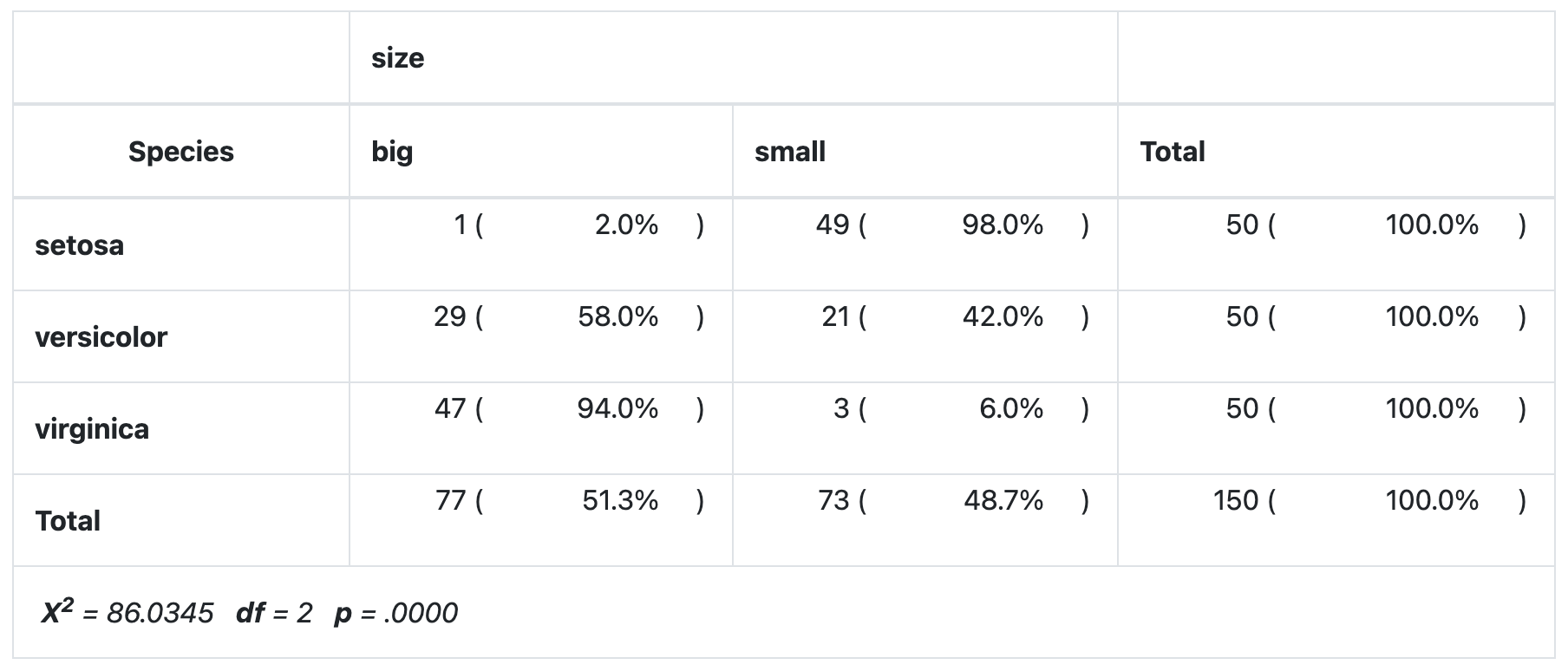
We now create a contingency table of the two variables Species and size with the table() function:
table(dat$Species, dat$size)

##
##              big small
##   setosa       1    49
##   versicolor  29    21
##   virginica   47     3
The contingency table gives the observed number of cases in each subgroup. For instance, there is only one big setosa flower, while there are 49 small setosa flowers in the dataset.
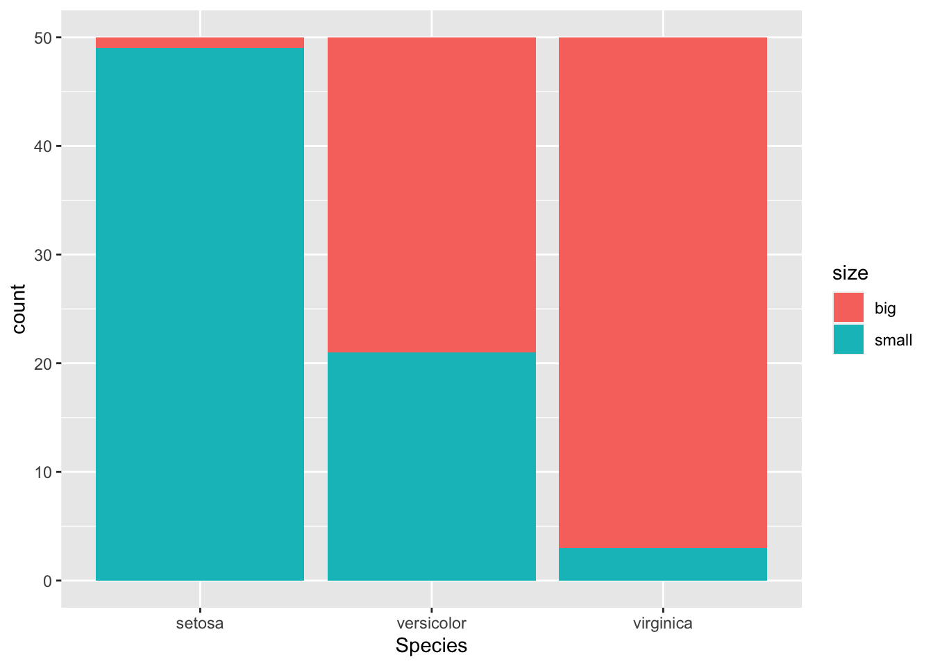
It is also a good practice to draw a barplot to visually represent the data:
library(ggplot2)
ggplot(dat) +
  aes(x = Species, fill = size) +
  geom_bar()
If you prefer to visualize it in terms of proportions (so that bars all have a height of 1, or 100%):
ggplot(dat) +
  aes(x = Species, fill = size) +
  geom_bar(position = "fill")
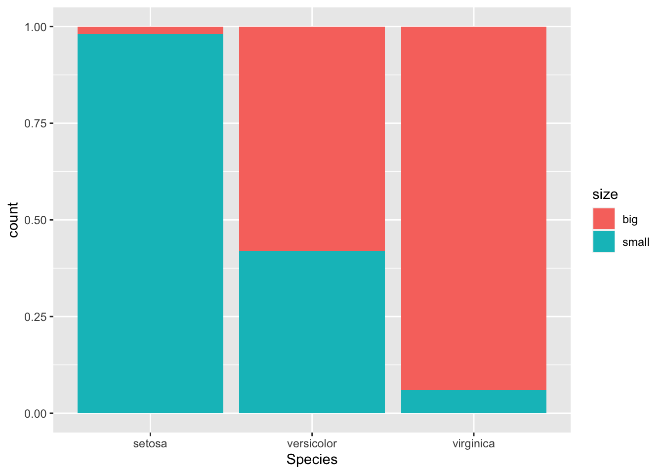
This second barplot is particularly useful if there are a different number of observations in each level of the variable drawn on the xxx-axis because it allows to compare the two variables on the same ground.
If you prefer to have the bars next to each other:
ggplot(dat) +
  aes(x = Species, fill = size) +
  geom_bar(position = "dodge")
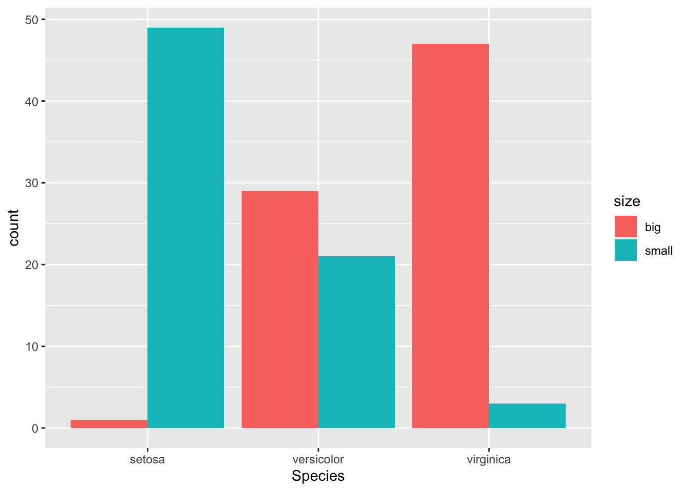
See the article “Graphics in R with ggplot2” to learn how to create this kind of barplot in {ggplot2}.
Chi-square test of independence in R
For this example, we are going to test in R if there is a relationship between the variables Species and size. For this, the chisq.test() function is used:
test <- chisq.test(table(dat$Species, dat$size))
test

##
##  Pearson's Chi-squared test
##
## data:  table(dat$Species, dat$size)
## X-squared = 86.035, df = 2, p-value < 2.2e-16
Everything you need appears in this output:
- the title of the test,
- which variables have been used,
- the test statistic,
- the degrees of freedom and
- the p-value of the test.
You can also retrieve the χ2 test statistic and the p-value with:
test$statistic

## X-squared
##  86.03451

test$p.value

## [1] 2.078944e-19
If you need to find the expected frequencies, use test$expected.
If a warning such as “Chi-squared approximation may be incorrect” appears, it means that the smallest expected frequencies is lower than 5. To avoid this issue, you can either:
- gather some levels (especially those with a small number of observations) to increase the number of observations in the subgroups, or
- use the Fisher’s exact test
The Fisher’s exact test does not require the assumption of a minimum of 5 expected counts in the contingency table. It can be applied in R thanks to the function fisher.test(). This test is similar to the Chi-square test in terms of hypothesis and interpretation of the results. Learn more about this test in this article dedicated to this type of test.
Talking about assumptions, the Chi-square test of independence requires that the observations are independent. This is usually not tested formally, but rather verified based on the design of the experiment and on the good control of experimental conditions. If you are not sure, ask yourself if one observation is related to another (if one observation has an impact on another). If not, it is most likely that you have independent observations.
If you have dependent observations (paired samples), the McNemar’s or Cochran’s Q tests should be used instead. The McNemar’s test is used when we want to know if there is a significant change in two paired samples (typically in a study with a measure before and after on the same subject) when the variables have only two categories. The Cochran’s Q tests is an extension of the McNemar’s test when we have more than two related measures.
For your information, there are three other methods to perform the Chi-square test of independence in R:
- with the
summary()function - with the
assocstats()function from the{vcd}package - with the
ctable()function from the{summarytools}package
# second method:
summary(table(dat$Species, dat$size))

## Number of cases in table: 150
## Number of factors: 2
## Test for independence of all factors:
##  Chisq = 86.03, df = 2, p-value = 2.079e-19

# third method:
vcd::assocstats(table(dat$Species, dat$size))

##                      X^2 df P(> X^2)
## Likelihood Ratio 107.308  2        0
## Pearson           86.035  2        0
##
## Phi-Coefficient   : NA
## Contingency Coeff.: 0.604
## Cramer's V        : 0.757

# fourth method:
library(summarytools)
library(dplyr)
dat %>%
  ctable(Species, size,
    prop = "r", chisq = TRUE, headings = FALSE
  ) %>%
  print(
    method = "render",
    style = "rmarkdown",
    footnote = NA
  )
As you can see all four methods give the same results.
If you do not have the same p-values with your data across the different methods, make sure to add the correct = FALSE argument in the chisq.test() function to prevent from applying the Yate’s continuity correction, which is applied by default in this method.1
Conclusion and interpretation
From the output and from test$p.value we see that the p-value is less than the significance level of 5%. Like any other statistical test, if the p-value is less than the significance level, we can reject the null hypothesis. If you are not familiar with p-values, I invite you to read this section.
In our context, rejecting the null hypothesis for the Chi-square test of independence means that there is a significant relationship between the species and the size. Therefore, knowing the value of one variable helps to predict the value of the other variable.
Combination of plot and statistical test
I recently discovered the mosaic() function from the {vcd} package. This function has the advantage that it combines a mosaic plot (to visualize a contingency table) and the result of the Chi-square test of independence:
library(vcd)

mosaic(~ Species + size,
  direction = c("v", "h"),
  data = dat,
  shade = TRUE
)
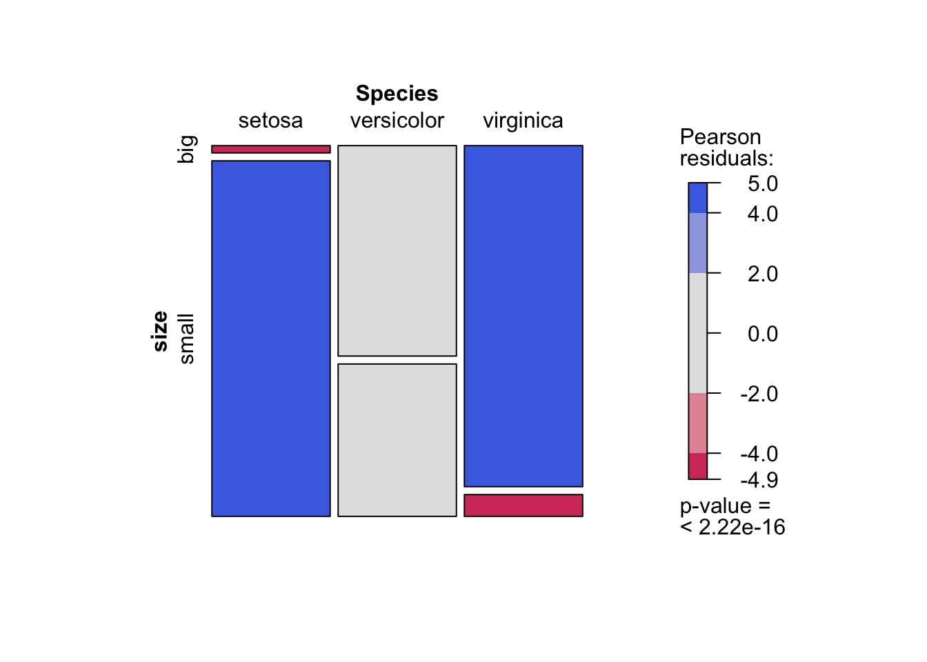
As you can see, the mosaic plot is similar to the barplot presented above, but the p-value of the Chi-square test is also displayed at the bottom right.
Moreover, this mosaic plot with colored cases shows where the observed frequencies deviates from the expected frequencies if the variables were independent. The red cases means that the observed frequencies are smaller than the expected frequencies, whereas the blue cases means that the observed frequencies are larger than the expected frequencies.
An alternative is the ggbarstats() function from the {ggstatsplot} package:
# load packages
library(ggstatsplot)
library(ggplot2)

# plot
ggbarstats(
  data = dat,
  x = size,
  y = Species
) +
  labs(caption = NULL) # remove caption
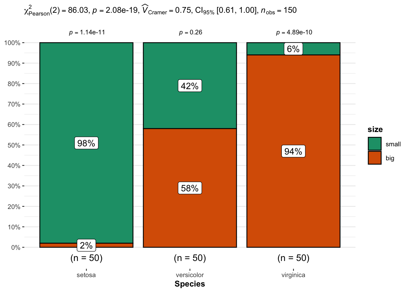
From the plot, it seems that big flowers are more likely to belong to the virginica species, while small flowers tend to belong to the setosa species. Species and size are thus expected to be dependent.
This is confirmed thanks to the statistical results displayed in the subtitle of the plot. There are several results, but we can in this case focus on the p-value which is displayed after p = at the top (in the subtitle of the plot).
As with the previous tests, we reject the null hypothesis and we conclude that species and size are dependent (p-value < 0.001).
Thanks for reading. I hope the article helped you to perform the Chi-square test of independence in R and interpret its results. If you would like to learn how to do this test by hand and how it works, read the article “Chi-square test of independence by hand”.
As always, if you have a question or a suggestion related to the topic covered in this article, please add it as a comment so other readers can benefit from the discussion.
Related articles
- ANOVA in R
- Wilcoxon test in R: how to compare 2 groups under the non-normality assumption
- Correlation coefficient and correlation test in R
- One-proportion and chi-square goodness of fit test
- How to do a t-test or ANOVA for more than one variable at once in R
16进制颜色设置透明度
https://blog.csdn.net/tabweb/article/details/107152141
对于RGB比较常见,显示器、电视等都是采用RGB的颜色标准。RGB是工业界的一种颜色标准,通过R(红)、G(绿)、B(蓝)三个颜色通道的变化以及它们相互之间的叠加来得到各式各样的颜色。我们知道计算机是0和1的世界,RGB每种色彩是用数字来表示,最大为255包括0,所以总共256级。所以RGB的色彩组合是256*256*256共16777216,一般简称千万色或者1600万,也有称为24位色,及2的24次方。在代码编程中常以16进制方式表示,如:0xff0000(红色)。
ARGB从表面看比RGB多了个A,也是一种色彩模式,是在RGB的基础上添加了Alpha(透明度)通道。透明度也是以0到255表示的,所以也是总共有256级,透明是0,不透明是255。代码编程中也是以16进制方式表示,如:0xffff0000。
- ARGB 依次代表透明度(alpha)、红色(red)、绿色(green)、蓝色(blue)。
- #FF99CC00 为例,其中,FF 是透明度,99 是红色值, CC 是绿色值, 00 是蓝色值。
- 透明度分为256阶(0-255),计算机上用16进制表示为(00-ff)。透明就是0阶,不透明就是255阶,如果50%透明就是127阶(256的一半当然是128,但因为是从0开始,所以实际上是127)。
- 透明度 和 不透明度 是两个概念, 它们加起来是1,或者100%.
透明度具体对应百分比:
100% — FF
 90% — E6
 80% — CC
 70% — B3
 60% — 99
 50% — 80
 40% — 66
 30% — 4D
 20% — 33
 10% — 1A
  0% — 00